Filter Response Curves
The data/filters/ subdirectory contains small files with tabulated filter
response curves. All files contain a single curve stored in the ASCII enhanced
character-separated value format, which is used
to specify the wavelength units and provide the following metadata:
Key |
Description |
|---|---|
group_name |
Name of the group that this filter response belongs to, e.g., sdss2010. |
band_name |
Name of the filter pass band, e.g., r. |
airmass |
Airmass used for atmospheric transmission, or zero for no atmosphere. |
url |
URL with more details on how this filter response was obtained. |
description |
Brief description of this filter response. |
The following sections summarize the standard filters included with the speclite
code distribution. Refer to the filters module API docs for
details and examples of how to load an use these filters. See
below for instructions on working with your own custom
filters.
SDSS Filters
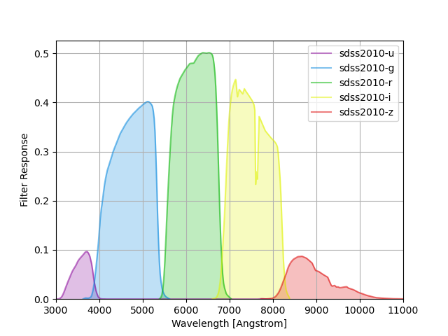
SDSS filter responses are taken from Table 4 of Doi et al, “Photometric Response Functions of the SDSS Imager”, The Astronomical Journal, Volume 139, Issue 4, pp. 1628-1648 (2010), and calculated as the reference response multiplied by the reference APO atmospheric transmission at an airmass 1.3. See the paper for details.
The group name sdss2010 is used to identify these response curves in
speclite. The plot below shows the output of:
sdss = speclite.filters.load_filters('sdss2010-*')
speclite.filters.plot_filters(sdss, wavelength_limits=(3000, 11000))
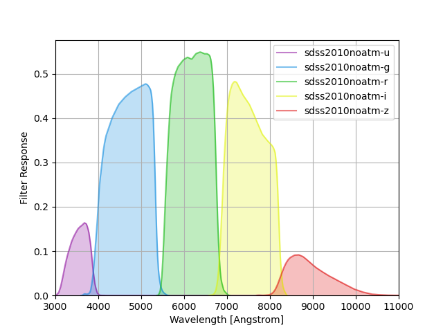
We also provide versions of the filters without the atmospheric transmission
which are identified by the sdss2010noatm group name and can be visualized
with this bit of code:
sdss_noatm = speclite.filters.load_filters('sdss2010noatm-*')
speclite.filters.plot_filters(sdss_noatm, wavelength_limits=(3000, 11000))
2MASS Filters
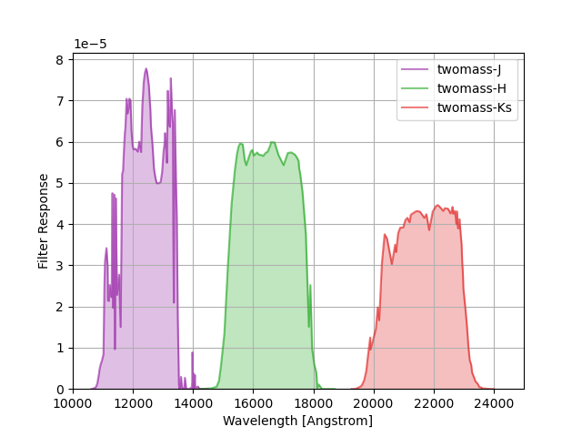
2MASS filter responses are taken from Cohen, Wheaton & Megeath, “Spectral Irradiance Calibration in the Infrared. XIV. The Absolute Calibration of 2MASS”, The Astronomical Journal, Volume 126, Issue 2, pp. 1090-1096 (2003), as tabulated by Michael Blanton. See the paper for details.
The group name twomass is used to identify these response curves in
speclite. The plot below shows the output of:
twomass = speclite.filters.load_filters('twomass-*')
speclite.filters.plot_filters(twomass, wavelength_limits=(10000, 25000))
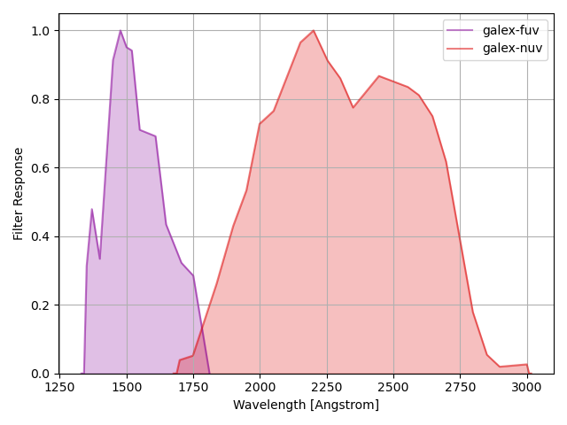
GALEX Filters
The command below produces the figure:
galex = speclite.filters.load_filters('galex-*')
speclite.filters.plot_filters(galex)
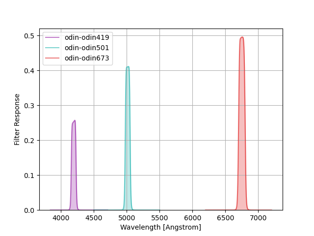
ODIN Narrow-band Filters
The One-hundred-deg2 DECam Imaging in Narrowbands (ODIN) survey filters consist of three narrow-band filters centered at (approximately) 419, 501, and 673 nm.
The command below produces the figure:
odin = speclite.filters.load_filters('odin-*')
speclite.filters.plot_filters(odin, legend_loc='upper left')
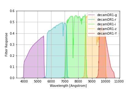
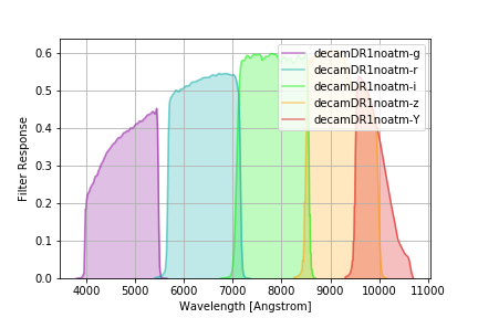
DECam DR1 Filters
The DECam DR1 filter curves are documented in T. M. C. Abbott et al 2018 ApJS 239 18 and available from this NSF NOIRLab DECam page. These represent the total system throughput and average instrumental response across the science CCDs. The official curves have arbitrary normalization, but the values used here have reasonable normalization factors applied for throughput calculations, provided by Douglas Tucker (Jan 2021, private communication).
There are two versions of the DR1 curves: decamDR1 with an airmass 1.2 reference atmosphere, and
decamDR1noatm with no atmospheric extinction:
with_atm = speclite.filters.load_filters('decamDR1-*')
speclite.filters.plot_filters(with_atm)
without_atm = speclite.filters.load_filters('decamDR1noatm-*')
speclite.filters.plot_filters(without_atm)
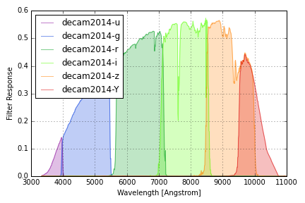
DECam 2014 Filters
The DECam 2014 filter responses are taken from this Excel spreadsheet created by William Wester in September 2014 and linked to this NSF NOIRLab DECam page. Throughputs include a reference atmosphere with airmass 1.3 provided by Ting Li. These are the most recent publicly available DECam throughputs as of Feb 2016.
The group name decam2014 is used to identify these response curves in
speclite. The plot below shows the output of:
decam = speclite.filters.load_filters('decam2014-*')
speclite.filters.plot_filters(
    decam, wavelength_limits=(3000, 11000), legend_loc='upper left')
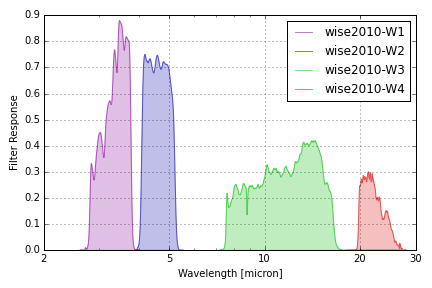
WISE Filters
WISE filter responses are taken from files linked to this page containing the weighted mean relative spectral responses described in Wright et al, “The Wide-field Infrared Survey Explorer (WISE): Mission Description and Initial On-orbit Performance”, The Astronomical Journal, Volume 140, Issue 6, pp. 1868-1881 (2010).
Note that these responses are based on pre-flight measurements but the in-flight responses of the W3 and W4 filters are observed to have effective wavelengths that differ by -(3-5)% and +(2-3)%, respectively. Refer to Section 2.2 of Wright et al. 2010 for details. See also Section 2.1.3 of Brown 2014 for further details about W4.
The group name wise2010 is used to identify these response curves in
speclite. The plot below shows the output of the command below, and matches
Figure 6 of the paper:
wise = speclite.filters.load_filters('wise2010-*')
speclite.filters.plot_filters(wise, wavelength_limits=(2, 30),
    wavelength_unit=astropy.units.micron, wavelength_scale='log')
plt.gca().set_xticks([2, 5, 10, 20, 30])
plt.gca().set_xticklabels([2, 5, 10, 20, 30])
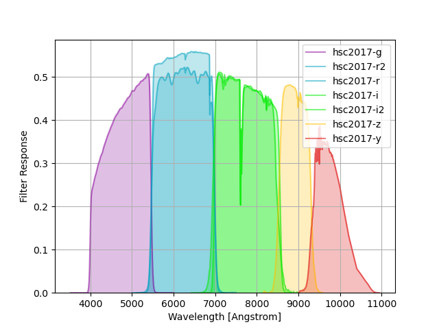
HSC Filters
HSC filter responses are taken from here, as described here and in Kawanamoto et al. 2018. These throughputs include a reference atmosphere with airmass 1.2.
The group name hsc2017 is used to identify these curves in speclite.
The plot below shows the output of the following command:
hsc = speclite.filters.load_filters('hsc2017-*')
speclite.filters.plot_filters(hsc)
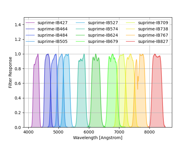
Suprime-Cam Intermediate-band Filters
Intermediate-band Suprime-Cam filters taken from here. The response is the total transmission, including the filter, the instrument, and the atmosphere.
The command below produces the figure:
suprime = speclite.filters.load_filters('suprime-*')
speclite.filters.plot_filters(suprime, legend_ncols=3, response_limits=[0, 1.5])
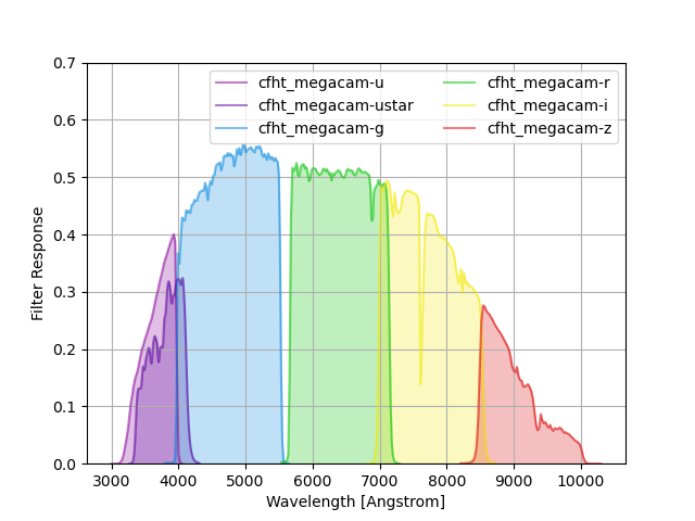
CFHT-MegaCam Filters
CFHT-MegaCam filters taken from here. The response is the total transmission, including the full telescope transmission (mirror+optics+CCD) plus 1.25 airmasses of atmospheric attenuation. Note that u* refers to the old (first-generation, through 2015) bandpass, whereas the u-band curve is the newer (post-2015, third-generation) filter curve.
The command below produces the figure:
megacam = speclite.filters.load_filters('cfht_megacam-*')
speclite.filters.plot_filters(megacam, legend_ncols=2, response_limits=[0, 0.7])
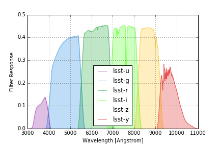
LSST (2016) Filters
LSST filter responses are taken from tag 12.0 of the LSST simulations throughputs package and include a standard atmosphere with airmass 1.2 that is also tabulated in the same package.
The group name lsst2016 is used to identify these response curves in speclite.
The plot below shows the output of the command below, and matches
Figure 6 of the paper:
lsst = speclite.filters.load_filters('lsst2016-*')
speclite.filters.plot_filters(
    lsst, wavelength_limits=(3000, 11000), legend_loc='upper left')
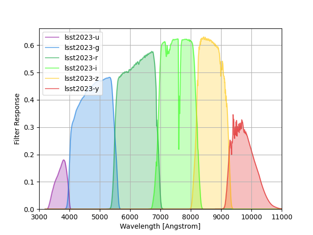
LSST (2023) Filters
LSST filter responses are taken from tag 1.9 of the LSST simulations throughputs package and include a standard atmosphere with airmass 1.2 that is also tabulated in the same package.
This tag follows the baselining of silver coatings on all three mirrors.
The group name lsst2023 is used to identify these response curves in speclite.
The plot below shows the output of the command below:
lsst = speclite.filters.load_filters('lsst2023-*')
speclite.filters.plot_filters(
    lsst, wavelength_limits=(3000, 11000), legend_loc='upper left')
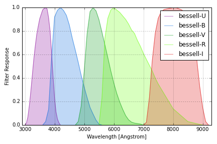
Johnson/Cousins Filters
Reference definitions of the Johnson/Cousins “standard” filters are taken from Table 2 of Bessell, M. S., “UBVRI passbands,” PASP, vol. 102, Oct. 1990, p. 1181-1199. We use the band name “U” for the response that Table 2 refers to as “UX”. Note that these do not represent the response of any actual instrument. Response values are normalized to have a maximum of one in each band.
The group name bessell is used to identify these response curves in
speclite. The plot below shows the output of the command below:
bessell = speclite.filters.load_filters('bessell-*')
speclite.filters.plot_filters(bessell, wavelength_limits=(2900, 9300))
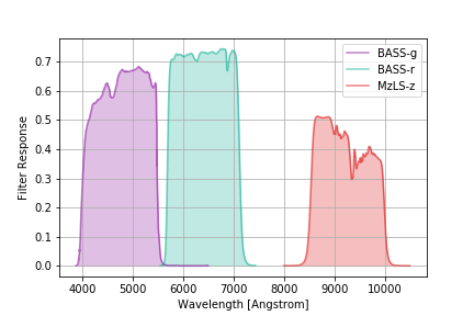
DESI Imaging Survey Filters
The DESI spectroscopic survey used imaging from the DECam, BASS and MzLS instruments to build its target catalog. The relevant BASS and MzLS filters are:
desi_imaging = speclite.filters.load_filters('BASS-g', 'BASS-r', 'MzLS-z')
speclite.filters.plot_filters(desi_imaging)
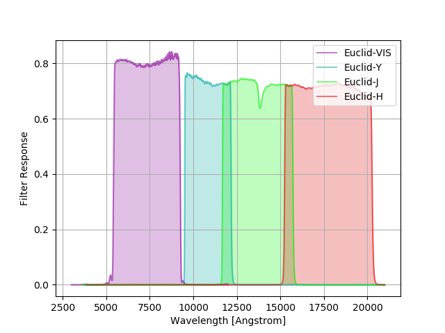
Euclid Filters
The current best end-of-life estimates for the “VIS”, “Y”, “H”, and “J” total throughputs for Euclid,
i.e., “Y”, “H”, and “J” have been convolved by the “NISP” throughput. The original tables can be found
here. The group name Euclid is used
to identify these curves in speclite.
The command below produces the figure:
euclid = speclite.filters.load_filters('Euclid-VIS', 'Euclid-Y', 'Euclid-H', 'Euclid-J')
speclite.filters.plot_filters(euclid)
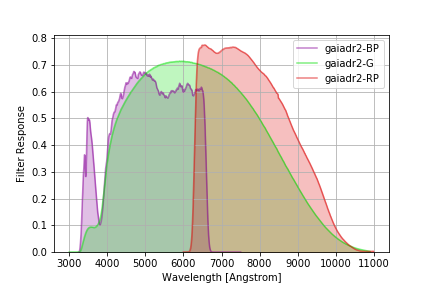
Gaia DR2 Filters
The (revised) filters from DR2 documented here.
The command below produces the figure:
gaiadr2 = speclite.filters.load_filters('gaiadr2-*')
speclite.filters.plot_filters(gaiadr2)
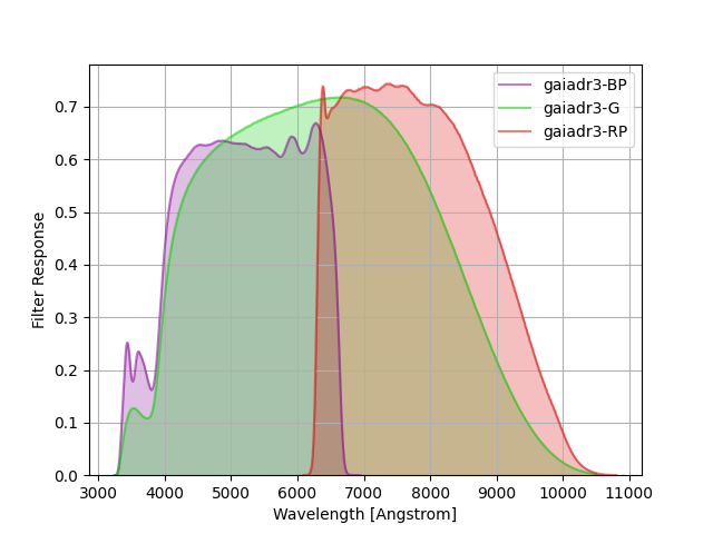
Gaia DR3 Filters
The filters from DR3/EDR3 documented here.
The command below produces the figure:
gaiadr3 = speclite.filters.load_filters('gaiadr3-*')
speclite.filters.plot_filters(gaiadr3)
Intermediate-Band Imaging Survey Filters
Intermediate-Band Imaging Survey (IBIS) filters taken from Arjun Dey (2024, private communication). The response is the total transmission, including the filter, the instrument, and the atmosphere at an airmass of 1.0.
The command below produces the figure:
ibis = speclite.filters.load_filters('ibis-*')
speclite.filters.plot_filters(ibis)

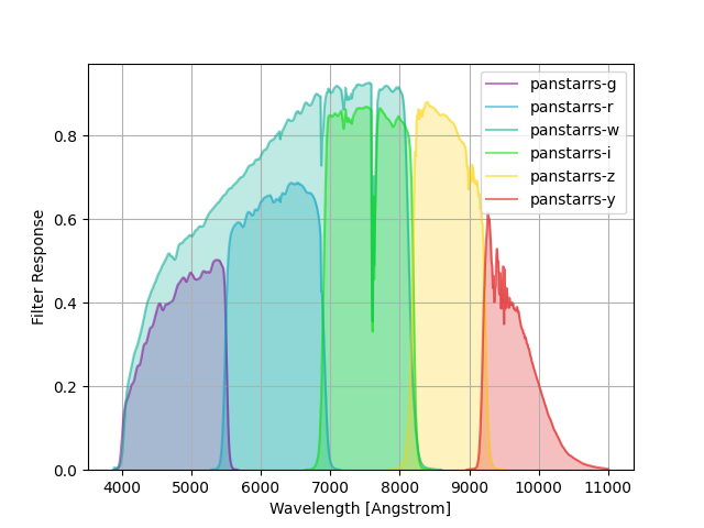
Pan-STARRS Filters
From Tonry et al. 2012, https://ui.adsabs.harvard.edu/abs/2012ApJ…750…99T/abstract
These are in units of square meters of cross section, at an airmass of 1.2 and PWV 0.65 cm and aerosol exponent 0.7 (quoting from the Fig 4 caption).
The command below produces the figure:
panstarrs = speclite.filters.load_filters('panstarrs-*')
speclite.filters.plot_filters(panstarrs)
Custom Filters
In addition to the standard filters included with the speclite code
distribution, you can create and read your own custom filters. For example
to define a new filter group called “fangs” with “g” and “r” bands, you
will first need to define your filter responses with new
speclite.filters.FilterResponse objects:
fangs_g = speclite.filters.FilterResponse(
    wavelength = [3800, 4500, 5200] * u.Angstrom,
    response = [0, 0.5, 0], meta=dict(group_name='fangs', band_name='g'))
fangs_r = speclite.filters.FilterResponse(
    wavelength = [4800, 5500, 6200] * u.Angstrom,
    response = [0, 0.5, 0], meta=dict(group_name='fangs', band_name='r'))
Your metadata dictionary must include the group_name and band_name
keys, but all of the keys listed above are recommended. You can now load and
use these filters with their canonical names, although the group wildcard
fangs-* is not supported. For example:
fangs = speclite.filters.load_filters('fangs-g', 'fangs-r')
speclite.filters.plot_filters(fangs)

Next, save these filters in the correct format to any directory:
directory_name = '.'
fg_name = fangs_g.save(directory_name)
fr_name = fangs_r.save(directory_name)
Note that the file name in the specified directory is determined automatically based on the filter’s group and band names.
Finally, you can now read these custom filters from other programs by
calling speclite.filters.load_filter() with paths:
directory_name = '.'
fg_name = os.path.join(directory_name, 'fangs-g.ecsv')
fr_name = os.path.join(directory_name, 'fangs-r.ecsv')
fangs_g = speclite.filters.load_filter(fg_name)
fangs_r = speclite.filters.load_filter(fr_name)
Note that load_filter and
load_filters
look for the “.ecsv” extension in the name to recognize a custom filter.