Reference/API
Operations on Spectroscopic Data
speclite.accumulate Module
Stack spectra on the same wavelength grid using weighted accumulation.
Functions
|
Combine the data from two spectra. |
speclite.downsample Module
Downsample spectra by combining adjacent pixels.
Functions
|
Downsample spectral data by a constant factor. |
speclite.resample Module
Resample spectra using interpolation.
Functions
|
Resample the data of one spectrum using interpolation. |
speclite.redshift Module
Apply redshift transformations to wavelength, flux, inverse variance, etc.
Functions
|
Transform spectral data from redshift z_in to z_out. |
Operations with Filters
speclite.filters Module
Support for calculations involving filter response curves.
Overview
See Filter Response Curves for information about the standard filters included with this code distribution and instructions for adding your own filters. Filter names have two components, a group name and a band name, which are combined with a hyphen, e.g. “sdss2010-r”. The group names included with this package are:
>>> filter_group_names
['sdss2010', 'sdss2010noatm', 'decam2014', 'wise2010', 'hsc2017', 'lsst2016', 'lsst2023', 'bessell', 'BASS', 'MzLS', 'Euclid', 'decamDR1', 'decamDR1noatm', 'gaiadr2', 'gaiadr3', 'twomass', 'galex', 'odin', 'suprime', 'cfht_megacam', 'ibis', 'panstarrs']
List the band names associated with any group using, for example:
>>> load_filters('sdss2010-*').names
['sdss2010-u', 'sdss2010-g', 'sdss2010-r', 'sdss2010-i', 'sdss2010-z']
Here is a brief example of calculating SDSS r,i and Bessell V magnitudes for a numpy array of fluxes for 100 spectra covering 4000-10,000 A with 1A pixels:
>>> import astropy.units as u
>>> wlen = np.arange(4000, 10000) * u.Angstrom
>>> flux = np.ones((100, len(wlen))) * u.erg / (u.cm**2 * u.s * u.Angstrom)
Units are recommended but not required (otherwise, the units shown here are assumed as defaults). Next, load the filter responses:
>>> import speclite.filters
>>> filters = speclite.filters.load_filters(
...     'sdss2010-r', 'sdss2010-i', 'bessell-V')
Finally, calculate the magnitudes to obtain an astropy Table of results with one row per input spectrum and one
column per filter:
>>> mags = filters.get_ab_magnitudes(flux, wlen)
If you prefer to work with a numpy structured array, you can convert the returned table:
>>> mags = filters.get_ab_magnitudes(flux, wlen).as_array()
Padding
Under certain circumstances, you may need to pad an input spectrum to cover
the full wavelength range of the filters you are using. See
FilterResponse.pad_spectrum() and FilterSequence.pad_spectrum() for
details on how this is implemented.
Shifted Filters
It can be useful to work with a filter whose wavelengths have been shifted,
e.g. for the applications
in http://arxiv.org/abs/astro-ph/0205243. This is supported with the
FilterResponse.create_shifted() method, for example:
>>> wlen = np.arange(4000, 10000) * u.Angstrom
>>> flux = np.ones(len(wlen)) * u.erg / (u.cm**2 * u.s * u.Angstrom)
>>> r0 = speclite.filters.load_filter('sdss2010-r')
>>> rz = r0.create_shifted(band_shift=0.2)
>>> print(np.round(r0.get_ab_magnitude(flux, wlen), 3))
-21.362
>>> print(np.round(rz.get_ab_magnitude(flux, wlen), 3))
-20.966
Note that a shifted filter has a different wavelength coverage, so may require padding of your input spectra.
Convolutions
The filter response convolution operator implemented here is defined as:
where \(R(\lambda)\) is a filter response function, represented by a
FilterResponse object, and \(f_\lambda \equiv dg/d\lambda\) is an
arbitrary differential function of wavelength, which can either be represented
as a callable python object or else with arrays of wavelengths and function
values.
The default weights:
are appropriate for photon-counting detectors such as CCDs, and enabled by
the default setting photon_weighted = True in the methods below. Otherwise,
the convolution is unweighted, \(\omega(\lambda) = 1\), but arbitrary
alternative weights can always be included in the definition of
\(f_\lambda\). For example, a differential function of frequency
\(dg/d\nu\) can be reweighted using:
These definitions make no assumptions about the units of \(f_\lambda\), but magnitude calculations are an important special case where the units of \(f_\lambda\) must have the dimensions \(M / (L T^3)\), for example, \(\text{erg}/(\text{cm}^2\,\text{s}\,\AA)\).
The magnitude of \(f_\lambda\) in the filter band with response \(R\) is then:
where \(f_{\lambda,0}(\lambda)\) is the reference flux density that defines the photometric system’s zeropoint \(F[R,f_{\lambda,0}]\). The zeropoint has dimensions \(1 / (L^2 T)\) and gives the rate of incident photons per unit telescope area from a zero magnitude source.
A spectral flux density per unit frequency, \(f_\nu = dg/d\nu\), should be converted using:
for use with the methods implemented here.
For the AB system,
and the convolutions use photon-counting weights.
Sampling
Filter responses are tabulated on non-uniform grids with sufficient sampling that linear interpolation is sufficient for most applications. When a filter response is convolved with tabulated data, we must also consider the sampling of the tabulated function. In this implementation, we assume that the tabulated function is also sufficiently sampled to allow linear interpolation.
The next issue is how to sample the product of a filter response and tabulated function when performing a numerical convolution integral. With the assumptions above, a safe strategy would be to sample the integrand at the union of the two wavelength grids. However, this is relatively expensive since it requires interpolating both the response and the input function. Interpolation is sometimes unavoidable: for example, when the function is linear and represented by its values at only two wavelengths.
The approach adopted here is to use the sampling grid of the input function to sample the convolution integrand whenever it samples the filter response sufficiently. This requires that the filter response be interpolated, but this operation only needs to be performed once when many convolutions are performed on the same input wavelength grid. Our criteria for sufficient filter sampling is that at most one filter wavelength point lies between any consecutive pair of input wavelength points. When this condition is not met, the input function will be interpolated at the minimum number of response wavelengths necessary to satisfy the condition.
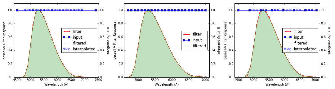
The figure below (generated by this function) illustrates three different sampling
regimes that can occur
in a convolution with the Bessell V filter (red curve). Filled blue squares
show where the input function is sampled and open blue circles show where
interpolation of the input function is performed. The left-hand plot shows
an extremely undersampled input that is interpolated at every filter point.
The middle plot shows a well sampled input that requires no interpolation.
The right-hand plot shows an input that is slightly undersampled and requires
interpolation at some of the filter points. All three methods give consistent
results, with discrepancies of < 0.05%.
The logic described here is encapsulated in the FilterConvolution
class. Interpolation is performed automatically, as necessary, by the
high-level magnitude calculating methods, but FilterConvolution is
available when more control of this process is needed to improve performance.
Performance
If the performance of magnitude calculations is a bottleneck, you can
speed up the code significantly by taking advantage of the fact that all
of the convolution functions can operate on multidimensional arrays. For
example, calling FilterResponse.get_ab_magnitudes() once with an
array of 5000 spectra is about 10x faster than calling it 5000 times with the
individual spectra. However, in order to take advantage of this speedup,
your spectra need to all use the same wavelength grid.
Note that the eliminating flux units (which are always optional) from your input spectra will only result in about a 10% speedup, so units are generally recommended.
Attributes
- filter_group_nameslist
List of filter group names included with this package.
- default_wavelength_unit
astropy.units.Unit The default wavelength units assumed when units are not specified. The same units are used to store wavelength values in internal arrays.
- default_flux_unit
astropy.units.Unit The default units for spectral flux density per unit wavelength.
Functions
|
Calculate an AB reference spectrum with the specified magnitude. |
|
Generate an explanatory plot for the documentation. |
|
Load a single filter response by name. |
|
Load a sequence of filters by name. |
|
Plot one or more filter response curves. |
|
Evaluate a function of wavelength. |
|
Validate a wavelength array for filter operations. |
Classes
|
Convolve a filter response with a tabulated function. |
|
A filter response curve tabulated in wavelength. |
|
Immutable sequence of filter responses. |
Other Functions
speclite.benchmark Module
Driver routines for benchmarking and profiling.
Functions
|
Run a suite of magnitude calclulations. |
|
Entry-point for speclite_benchmark. |
speclite.utils Package
Functions
|
convenience wrapper to return location of data file |